Background
There are several barriers to using OpenFOAM for research in the dust explosion field. For practitioners interested in simulating specific problems, a lack of documentation makes problem setup and interpretation of the results difficult. For researchers experienced in Computational Fluid Dynamics (CFD), the highly object-oriented nature of the source code makes it difficult to track down specific calculation routines. To aid researchers in this area, the current post gives an overview of the code structure for reactive Lagrangian particles in CoalChemistryFoam. The information given in this post is also relevant to other solvers using reactive Lagrange tracking such as reactiveParcelFoam and sprayFoam.
Flow Chart Development
Trudging through individual class definitions in OpenFoam is often a time consuming and frustrating task. I will say a few words on the approach I used here, as it may be helpful to others. In the source code hierarchy each class declaration and definition is generally contained in a folder with the name of that class. To construct a flow chart of the Lagrange code structure, a one page summary of each class was created which contains the classes it includes, any input taken from problem setup files, and a summary of any important functions. The embedded search functionality in folder viewer and the Grep Terminal Command are invaluable tools for sifting through the openFoam/src directory. For example the command [grep -r -e “include \”Cloud.H\””] will search the whole directory for any files that include Cloud.H.
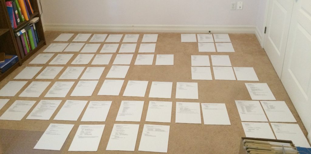
Once the one page summaries for each class are created, they can be organized to determine the overall structure of the class definitions. This is best done by laying out the class descriptions on a flat surface as shown in the following image and reordering them until the overall organization can be determined. The process of summarizing all of the Lagrange class definitions and organizing the flow chart took about three days of effort.
Digital Flow Chart
A digital version of the code flow chart was developed in LibreOffice Draw and is shown in the following image. A PDF version for printing can be accessed by clicking the image or the link here. The arrows in the flow chart show classes that include each other and give an idea of the classes responsible for different code routines (this is described in more detail below)
The starting point for the Lagrangian cloud definition is in the coalCloud class (see coalCloud.H). In this file coalCloud is templated from the KinematicCloud, ThermoCloud, ReactingCloud, and ReactingMultiphaseCloud classes and inherits their functionality. Each of these template classes are responsible for different parts of the Lagrange treatment and their resulting class hierarchy are indicated by different colors in the image. The four main template classes are shown in red, blue, purple, and green. The black blocks are high level base classes used for C++ setup, and do not generally contain any of the computational routines. The orange boxes are for Solid-Liquid-Gas thermodynamic parameters (SLGThermo) for particles containing both solid, liquid, and gas components. The OpenFOAM Lagrange hierarchy contains three main elements: individual particles, parcels (groups of particles), and clouds (groups of parcels), of which there are classes specifically for clouds and parcels.
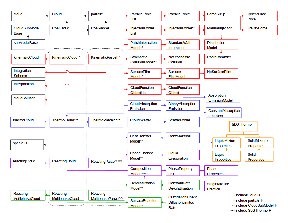
The terminal elements to the right in the flow chart are models used for calculating the physical processes for Lagrange parcels (i.e., physical models). The specific models included in the flow chart are those used in the simplifiedSiwek tutorial for coalChemistryFoam (e.g., SphereDragForce, gravityForce, etc.). However, coalChemistryFoam also has many other options that can be used for these physical models.
Physical Model Summary
A summary of the physical models available for OpenFOAM 3.0.1 is given in the following list. The color coding is the same as in the flow chart above, and a pdf of the list can be accessed here. In general the kinematicCloud class is responsible for particle motion and initialization, the thermoCloud class for particle heating, the reactingCloud class for liquid evaporation and phase change, and the reactingMultiphaseCloud class for solid particle surface reaction and devolatilization. The physical models in the image are underlined and the different options available are listed underneath them. The arrows to the right of the models indicate those used in the simplifiedSiwek tutorial (described further below).
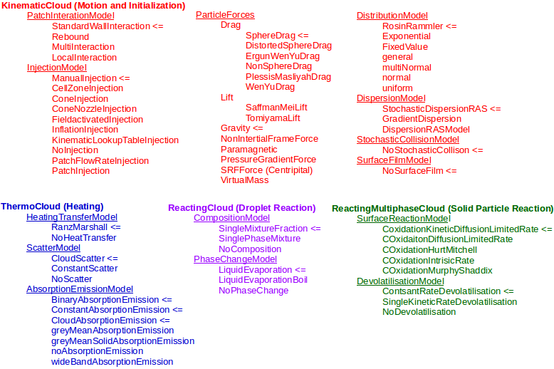
In the simplifiedSiwek tutorial the kinematic physical models include StandardWallInteraction, ManualInjection, SphereDragForce, gravityForce, RosinRammler distribution, and StochasticDispersion based on RANS turbulence. The standard wall interaction is perfectly elastic and manual injection places particles at defined locations (see [cloudName]positions) at the start of the simulation. A spherical drag force and gravity acts on the particles (however, note that the fluid solver for coalChemistryFoam does not include gravity).
The thermal physical models include RanzMarshall heating (based on the particle Sherwood Number) as well as Thermal Radiation. Radiative scattering from the particle cloud is included (CloudScatter) along with a binaryAbsorptionEmission model which includes effects from both the background fluid and particle cloud (constantAbsorptionEmission and CloudAbsorptionEmission, respectively).
Both the reactingCloud and reactingMultiphaseCloud classes are used in coalChemistryFoam. The coal particles are made up of solid, liquid, and gas components, and use the most general composition approach (SingelMixtureFraction). Evaporation of the liquid components to the gas phase is captured using the LiquidEvaporaton class. Surface reaction uses a diffusion or kinetic limited model, while devolatilization is simulated using a constant rate approach.
Future Posts
Hopefully, this post and the attached material have helped explain the setup of Lagrange classes and the physical models available in coalChemistryFoam. If you have any questions or comments please do not hesitate to comment below. Future posts will focus on the different simulation input parameters and how they are used, and determining the computational process that the Lagrange parcels go through during the calculation. Further work is also being completed on characterizing the fluid solver, thermophysical models, and combustion routines.